Quick Start Guide
This page provides simple quick-start information for using sangeranalyseR with AB1 files. Please read the Beginners Guide page for more details on each step.
If you haven’t already, please follow the steps in the Installation page to install and load sangeranalyseR.
Super-Quick Start (3 lines of code)
The most minimal example gets the job done in three lines of code. More details below.
my_aligned_contigs <- SangerAlignment(ABIF_Directory      = "./my_data/",
                                      REGEX_SuffixForward = "_[0-9]*_F.ab1$",
                                      REGEX_SuffixReverse = "_[0-9]*_R.ab1$")

writeFasta(my_aligned_contigs)

generateReport(my_aligned_contigs)
Step 1: Prepare your input files
Put all your AB1 files in a directory ./my_data/. The directory can be called anything.
Name your files according to the convention contig_index_direction.ab1. E.g. Drosophila_COI_1_F.ab1 and Drosophila_COI_2_R.ab1 describes a forward and reverse read to assemble into one contig. You can have as many files and contigs as you like in one directory.
Step 2: Load and analyse your data
my_aligned_contigs <- SangerAlignment(ABIF_Directory      = "./my_data/",
                                      REGEX_SuffixForward = "_[0-9]*_F.ab1$",
                                      REGEX_SuffixReverse = "_[0-9]*_F.ab1$")
This command loads, trims, builds contigs, and aligns contigs. All of these are done with sensible default values, which can be changed. I
Step 3 (optional): Explore your data
launchApp(my_aligned_contigs)
This launches an interactive Shiny app where you can view your analysis, change the default settings, etc.
Step 4: Output your aligned contigs
writeFasta(my_aligned_contigs)
This will save your aligned contigs as a FASTA file.
Step 5 (optional): Generate an interactive report
generateReport(my_aligned_contigs)
This will save a detailed interactive HTML report that you can explore.
A Reproducible Example
If you are still confused about how to run sangeranalyseR and want to check whether it produces the results that you want, then check this section for more details. Here we demonstrate a simple and reproducible example for using sangeranalyseR to generate a consensus read from 8 sanger ab1 files (4 contigs and each includes a forward and a reverse read).
1. Prepare your input files & loading
The data of this example is in the sangeranalyseR package; thus, you can simply get its path from the library.
rawDataDir <- system.file("extdata", package = "sangeranalyseR")
parentDir <- file.path(rawDataDir, 'Allolobophora_chlorotica', 'ACHLO')
2. Load and analyse your data
Run the following on-liner to create the sanger alignment object.
ACHLO_contigs <- SangerAlignment(ABIF_Directory     = parentDir,
                                 REGEX_SuffixForward = "_[0-9]*_F.ab1$",
                                 REGEX_SuffixReverse = "_[0-9]*_R.ab1$")
3. Explore your data
Launch the Shiny app to check the visualized results.
launchApp(ACHLO_contigs)
And a Shiny would popup as showed in Figure 1
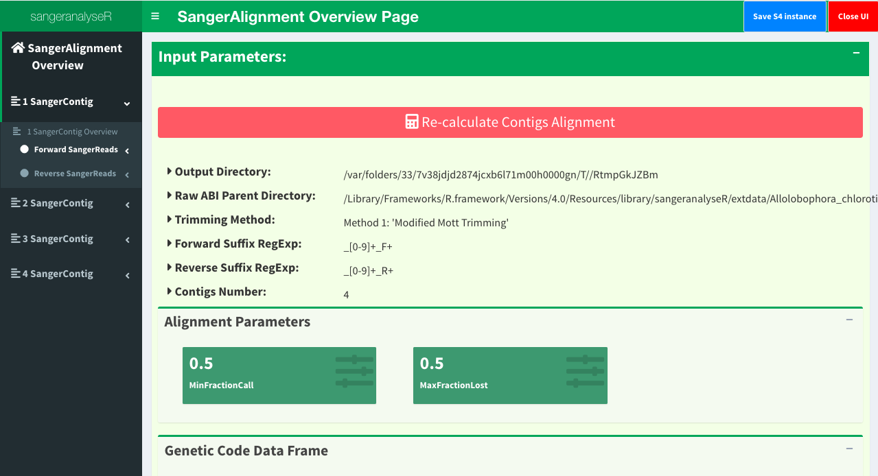
Figure 1. SangerAlignment Shiny dashboard.
4. Output your aligned contigs
Write each contig and the aligned consensus read into FASTA files.
writeFasta(ACHLO_contigs)
And you will get three FASTA files:
5. Generate an interactive report
Last but not least, generate an Rmarkdown report to store all the sequence information.
generateReport(ACHLO_contigs)
For more detailed analysis steps, please choose one the following topics :